Elementary Data Structures
Elementary Data Structures
Name: - Sanjyot Sanjay Mankar
Urn no: - 2020-B-03022003
Class: - BCA CTMA
Course Name: - Data structure using C.
- Abstract Data Type & Array in C++:
- Abstract Data type: -
- The Data Type is basically a type of data that can be used in a different computer program. It signifies the type like integer, float, etc, the space-like integer will take 4-bytes, a character will take 1-byte of space, etc.
- The abstract data type is a special kind of datatype, whose behavior is defined by a set of values and a set of operations. The keyword “Abstract” is used as we can use these data types, we can perform different operations.
- But how those operations are working is totally hidden from the user. The ADT is made of primitive data types, but operation logics are hidden. Some examples of ADT are Stack, Queue, List, etc.
- Element − Each item stored in an array is called an element.
- Index − Each location of an element in an array has a numerical index, which is used to identify the element.
")
- C++ provides a data structure, the array, which stores a fixed-size sequential collection of elements of the same type. An array is used to store a collection of data, but it is often more useful to think of an array as a collection of variables of the same type.
- Instead of declaring individual variables, such as number0, number1, ..., and number99, you declare one array variable such as numbers and use numbers[0], numbers[1], and ..., numbers[99] to represent individual variables. A specific element in an array is accessed by an index.
- All arrays consist of contiguous memory locations. The lowest address corresponds to the first element and the highest address to the last element.
type arrayName [ arraySize ];
- Introduction to stack and queue: -
- Implementation of the list with an array:-
- This implementation stores the list in an array.
- The position of each element is given by an index from 0 to n-1, where n is the number of elements.
- The element with the index can be accessed in constant time (ie) the time to access does not depend on the size of the list.
- The time taken to add an element at the end of the list does not depend on the size of the list. But the time taken to add an element at any other point in the list depends on the size of the list because the subsequent elements must be shifted to the next index value. So the additions near the start of the list take a longer time than the additions near the middle or end.
- A stack is an Abstract Data Type (ADT), commonly used in most programming languages.
- Stack ADT allows all data operations at one end only. At any given time, we can only access the top element of a stack. This feature makes it LIFO data structure. LIFO stands for Last-in-first-out. Here, the element which is placed (inserted or added) last, is accessed first. In stack terminology, insertion operation is called PUSH operation, and removal operation is called POP operation.
Stack Representation: -

- Basic Operations: -
- push() − Pushing (storing) an element on the stack.
- pop() − Removing (accessing) an element from the stack.
- peek() − get the top data element of the stack, without removing it.
- isFull() − check if stack is full.
- isEmpty() − check if stack is empty.
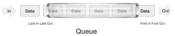
- A queue is an abstract data structure, somewhat similar to Stacks. Unlike stacks, a queue is open at both ends. One end is always used to insert data (enqueue) and the other is used to remove data (dequeue). Queue follows First-In-First-Out methodology, i.e., the data item stored first will be accessed first.
- As we now understand that in the queue, we access both ends for different reasons. The following diagram given below tries to explain queue representation as data structure −
- Basic Operations:
- enqueue() − add (store) an item to the queue.
- dequeue() − remove (access) an item from the queue.
- peek() − Gets the element at the front of the queue without removing it.
- isfull() − Checks if the queue is full.
- isempty() − Checks if the queue is empty.
- Pointer and References in c++: -
1.
Review of Pointer: -- Just
like integers and characters, a pointer is a primitive
data type in C/C++.
- An
integer takes up 4 bytes, a character takes up 1 byte, and a pointer takes up 4
bytes on a 32-bit machine (and 8 bytes on a 64-bit machine, but we will assume
that we are running on a 32-bit machine for the rest of this discussion).
- A
pointer is simply a 4-byte quantity that contains a memory address. Here's
an example of how you would declare an integer variable, a character variable,
and a pointer variable in C:
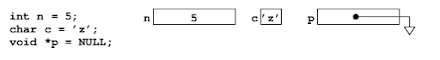
Fig (3) Intro to pointer
- n = 5 means to put an integer value of 5 into the
memory location referred to by n. c = 'z' means to put an
encoded character 'Z into the memory location referred to
by c. p = NULL means to put a value of 0 into the
memory location referred to by p since NULL is simply
defined as 0.
2. C-Pointers: -
- A pointer is a variable whose value is the address of another variable, i.e., the direct address of the memory location. Like any variable or constant, you must declare a pointer before using it to store any variable address. The general form of a pointer variable declaration is −
type *var-name;
- Here, type is the pointer's base type; it must be a valid C data type and var-name is the name of the pointer variable. The asterisk * used to declare a pointer is the same asterisk used for multiplication. However, in this statement, the asterisk is being used to designate a variable as a pointer. Take a look at some of the valid pointer declarations −
int    *ip;    /* pointer to an integer */
double *dp;    /* pointer to a double */
float  *fp;    /* pointer to a float */
char   *ch     /* pointer to a character */
- Just like integers and characters, a pointer is a primitive data type in C/C++.
- An integer takes up 4 bytes, a character takes up 1 byte, and a pointer takes up 4 bytes on a 32-bit machine (and 8 bytes on a 64-bit machine, but we will assume that we are running on a 32-bit machine for the rest of this discussion).
- A pointer is simply a 4-byte quantity that contains a memory address. Here's an example of how you would declare an integer variable, a character variable, and a pointer variable in C:
Fig (3) Intro to pointer
- n = 5 means to put an integer value of 5 into the memory location referred to by n. c = 'z' means to put an encoded character 'Z into the memory location referred to by c. p = NULL means to put a value of 0 into the memory location referred to by p since NULL is simply defined as 0.
2. C-Pointers: -
- A pointer is a variable whose value is the address of another variable, i.e., the direct address of the memory location. Like any variable or constant, you must declare a pointer before using it to store any variable address. The general form of a pointer variable declaration is −
type *var-name;
- Here, type is the pointer's base type; it must be a valid C data type and var-name is the name of the pointer variable. The asterisk * used to declare a pointer is the same asterisk used for multiplication. However, in this statement, the asterisk is being used to designate a variable as a pointer. Take a look at some of the valid pointer declarations −
int *ip; /* pointer to an integer */ double *dp; /* pointer to a double */ float *fp; /* pointer to a float */ char *ch /* pointer to a character */
- Simple Program: -
#include
<stdio.h>
int main ()
{
int var =60;
int *ip;
ip =
&var;
printf("Address of var variable: %x\n", &var );
printf("Address stored in ip variable: %x\n", ip );
printf("Value of *ip variable: %d\n", *ip );
return
0;
}
- After run, this program Output gives like this: -
Address of var
variable: cd880e6c
Address stored in ip
variable: cd880e6c
Value of *ip variable:
60
- There may be a situation when we want to maintain an array, which can store pointers to an int or char or any other data type available. Following is the declaration of an array of pointers to an integer −
int *ptr[MAX];
- It declares ptr as an array of MAX integer pointers. Thus, each element in ptr, holds a pointer to an int value. The following example uses three integers, which are stored in an array of pointers, as follows −
- Simple Program: -
#include
<stdio.h>
const int MAX = 3;
int main ()
{
int
var[] = {19, 38, 57};
int i, *ptr[MAX];
for ( i = 0; i < MAX; i++)
{
ptr[i] = &var[i];
}
for ( i = 0; i < MAX; i++) {
printf("Value of var[%d] =
%d\n", i, *ptr[i] );
}
return 0;
}
- After Run this program the Output gives like this: -
Value of var[0] = 19
Value of var[1] = 38
Value of var[2] = 57
- Dynamic Memory Allocation: -
- Dynamic memory allocation: -
- memory is allocated at run time.
- memory can be increased while executing program.
- used in linked list.
2 . Dynamic memory allocation in C: -
- It is possible by 4 functions :
- malloc()
- calloc()
- realloc()
- free()
The syntax of malloc() function is given below:
1. ptr=(cast-type*)malloc(byte-size)
Let's see the example of malloc() function.
#include<stdio.h>
#include<stdlib.h>
int main(){
int
n,i,*ptr,sum=0;
printf("Enter number of elements: ");
scanf("%d",&n);
ptr=(int*)malloc(n*sizeof(int));
if(ptr==NULL)
{
printf("Sorry! unable to allocate memory");
exit(0);
}
printf("Enter elements of array: ");
for(i=0;i<n;++i)
{
scanf("%d",ptr+i);
sum+=*(ptr+i);
}
printf("Sum=%d",sum);
free(ptr);
return 0;
}
- After running this program output gives like this: -
Enter elements of
array: 3
Enter elements of array: 10
10
10
Sum=30
- The syntax of calloc() function is given below:
1. ptr=(cast-type*)calloc(number, byte-size)
- Let's see the syntax of realloc() function.
1.
ptr=realloc(ptr, new-size)
- Let's see the syntax of free() function.
1. free(ptr)
All these 4 functions output is same just changing the function.
- Dynamic memory Allocation in C++: -
- How dynamic memory really works in C++ is essential to becoming a good C++ programmer. Memory in your C++ program is divided into two parts −
- The stack − All variables declared inside the function will take up memory from the stack.
- The heap − This is unused memory of the program and can be used to allocate the memory dynamically when program runs.
- Many times, you are not aware in advance how much memory you will need to store particular information in a defined variable and the size of required memory can be determined at run time.
- You can allocate memory at run time within the heap for the variable of a given type using a special operator in C++ which returns the address of the space allocated. This operator is called new operator.
- If you are not in need of dynamically allocated memory anymore, you can use delete operator, which de-allocates memory that was previously allocated by new operator.
- There is following generic syntax to use new operator to allocate memory dynamically for any data-type.
new data-type;
- Here, data-type could be any built-in data type including an array or any user defined data types include class or structure. Let us start with built-in data types. For example we can define a pointer to type double and then request that the memory be allocated at execution time. We can do this using the new operator with the following statements −
double* pvalue  = NULL; // Pointer initialized with null
pvalue  = new double;   // Request memory for the variable
- The memory may not have been allocated successfully, if the free store had been used up. So it is good practice to check if new operator is returning NULL pointer and take appropriate action as below −
double* pvalue  = NULL;
if( !(pvalue  = new double )) {
   cout << "Error: out of memory." <<endl;
   exit(1);
}
- The malloc() function from C, still exists in C++, but it is recommended to avoid using malloc() function. The main advantage of new over malloc() is that new doesn't just allocate memory, it constructs objects which is prime purpose of C++.
- At any point, when you feel a variable that has been dynamically allocated is not anymore required, you can free up the memory that it occupies in the free store with the ‘delete’ operator as follows −
delete pvalue; // Release memory pointed to by pvalue
#include<iostream>
using namespace std;
int main ()
{
double*
pvalue = NULL; // Pointer initialized
with null
pvalue = new double; // Request memory for the variable
*pvalue =
29494.99; // Store value at allocated
address
cout << "Value of pvalue : " << *pvalue << endl;
delete pvalue; // free up the memory.
return 0;
}
Value of pvalue : 29495
- Linked stacks, queues, lists: -
- Link list: -
- Link list: -
- A linked list is a linear data structure, in which the elements are not stored at contiguous memory locations. The elements in a linked list are linked using pointers as shown in the below image:

- In simple words, a linked list consists of nodes where each node contains a data field and a reference(link) to the next node in the list.
- A linked list is a sequence of data structures, which are connected together via links. Linked List is a sequence of links which contains items. Each link contains a connection to another link. Linked list is the second most-used data structure after array.
2. Link Stacks: -
- instead of using array, we can also use linked list to implement stack. Linked list allocates the memory dynamically. However, time complexity in both the scenario is same for all the operations i.e. push, pop and peek.
- In linked list implementation of stack, the nodes are maintained non-contiguously in the memory. Each node contains a pointer to its immediate successor node in the stack. Stack is said to be overflown if the space left in the memory heap is not enough to create a node.
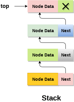
- The top most node in the stack always contains null in its address field. Lets discuss the way in which, each operation is performed in linked list implementation of stack.
- Implementaion of stack in link list in C: -
#include <stdio.h>
#include <stdlib.h>
void push();
void pop();
void display();
struct node
{
int val;
struct node *next;
};
struct node *head;
void main ()
{
int
choice=0;
while(choice !=
4)
{
printf("\n\nChose one from the below options...\n");
printf("\n1.Push\n2.Pop\n3.Show\n4.Exit");
printf("\n Enter your choice \n");
scanf("%d",&choice);
switch(choice)
{
case
1:
{
push();
break;
}
case
2:
{
pop();
break;
}
case 3:
{
display();
break;
}
case
4:
{
printf("Exiting....");
break;
}
default:
{
printf("Please Enter valid choice ");
}
};
}
}
void push ()
{
int val;
struct node *ptr
= (struct node*)malloc(sizeof(struct node));
if(ptr ==
NULL)
{
printf("not able to push the element");
}
else
{
printf("Enter the value");
scanf("%d",&val);
if(head==NULL)
{
ptr->val = val;
ptr ->
next = NULL;
head=ptr;
}
else
{
ptr->val = val;
ptr->next = head;
head=ptr;
}
printf("Item pushed");
}
}
void pop()
{
int item;
struct node
*ptr;
if (head ==
NULL)
{
printf("Underflow");
}
else
{
item =
head->val;
ptr =
head;
head =
head->next;
free(ptr);
printf("Item popped");
}
}
void display()
{
int i;
struct node
*ptr;
ptr=head;
if(ptr ==
NULL)
{
printf("Stack is empty\n");
}
else
{
printf("Printing Stack elements \n");
while(ptr!=NULL)
{
printf("%d\n",ptr->val);
ptr =
ptr->next;
}
}
}
Chose one from the below options...
1.Push
2.Pop
3.Show
4.Exit
Enter your choice
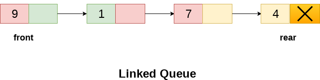
- In a linked queue, each node of the queue consists of two parts i.e. data part and the link part. Each element of the queue points to its immediate next element in the memory.
- In the linked queue, there are two pointers maintained in the memory i.e. front pointer and rear pointer. The front pointer contains the address of the starting element of the queue while the rear pointer contains the address of the last element of the queue.
- Insertion and deletions are performed at rear and front end respectively. If front and rear both are NULL, it indicates that the queue is empty.
- The linked representation of queue is shown in the following figure.
- Implementing link queued in C: -
#include<stdio.h>
#include<stdlib.h>
struct node
{
int data;
struct node
*next;
};
struct node *front;
struct node *rear;
void insert();
void delete();
void display();
void main ()
{
int choice;
while(choice !=
4)
{
printf("\nMain Menu\n");
printf("\n1.insert an element\n2.Delete an element\n3.Display the
queue\n4.Exit\n");
printf("\nEnter your choice =");
scanf("%d",& choice);
switch(choice)
{
case
1:
insert();
break;
case
2:
delete();
break;
case
3:
display();
break;
case
4:
exit(0);
break;
default:
printf("\nEnter valid choice??\n");
}
}
}
void insert()
{
struct node
*ptr;
int item;
ptr = (struct
node *) malloc (sizeof(struct node));
if(ptr ==
NULL)
{
printf("\nOVERFLOW\n");
return;
}
else
{
printf("\nEnter value?\n");
scanf("%d",&item);
ptr ->
data = item;
if(front ==
NULL)
{
front = ptr;
rear =
ptr;
front
-> next = NULL;
rear
-> next = NULL;
}
else
{
rear
-> next = ptr;
rear =
ptr;
rear->next = NULL;
}
}
}
void delete ()
{
struct node
*ptr;
if(front ==
NULL)
{
printf("\nUNDERFLOW\n");
return;
}
else
{
ptr =
front;
front = front
-> next;
free(ptr);
}
}
void display()
{
struct node
*ptr;
ptr = front;
if(front ==
NULL)
{
printf("\nEmpty queue\n");
}
else
{ printf("\nprinting values
.....\n");
while(ptr !=
NULL)
{
printf("\n%d\n",ptr -> data);
ptr = ptr
-> next;
}
}
}
Main Menu
1.insert an element
2.Delete an element
3.Display the queue
4.Exit
Enter your choice =
- Algorithm Efficiency: -
- algorithm
efficiency A measure of the average execution time necessary for an
algorithm to complete work on a set of data. Algorithm efficiency is
characterized by its order.
- Typically
a bubble sort algorithm will have efficiency in sorting N items
proportional to and of the order of N2, usually written O(N2).
- This is because an average of N/2
comparisons are required N/2 times, giving N2/4 total comparisons,
hence of the order of N2. In contrast, quicksort has an
efficiency O(N log2N).
-
If two algorithms for the same problem are of the same order then they are
approximately as efficient in terms of computation. Algorithm efficiency is
useful for quantifying the implementation difficulties of certain problems
- Searching and Sorting Algorithms: -
1.Searching Algorithm: -
- algorithm efficiency A measure of the average execution time necessary for an algorithm to complete work on a set of data. Algorithm efficiency is characterized by its order.
- Typically a bubble sort algorithm will have efficiency in sorting N items proportional to and of the order of N2, usually written O(N2).
- This is because an average of N/2 comparisons are required N/2 times, giving N2/4 total comparisons, hence of the order of N2. In contrast, quicksort has an efficiency O(N log2N).
- If two algorithms for the same problem are of the same order then they are approximately as efficient in terms of computation. Algorithm efficiency is useful for quantifying the implementation difficulties of certain problems
- Searching and Sorting Algorithms: -
- A search algorithm is a step-by-step procedure used to locate specific data among a collection of data. It is considered a fundamental procedure in computing. In computer science, when searching for data, the difference between a fast application and a slower one often lies in the use of the proper search algorithm.
- To search an element in a given array, there are two popular algorithms available:
1.Linear Search
2.Binary Search
1]Linear Search
- Linear search is a very basic and simple search algorithm. In Linear search, we search an element or value in a given array by traversing the array from the starting, till the desired element or value is found.
- It compares the element to be searched with all the elements present in the array and when the element is matched successfully, it returns the index of the element in the array, else it returns -1.
- Linear Search is applied on unsorted or unordered lists, when there are fewer elements in a list.
- Features of Linear Search Algorithm
- It is used for unsorted and unordered small list of elements.
- It has a time complexity of O(n), which means the time is linearly dependent on the number of elements, which is not bad, but not that good too.
- It has a very simple implementation.
- ·
Binary
Search is used with sorted array or list. In binary search, we follow the
following steps:
- ·
We
start by comparing the element to be searched with the element in the middle of
the list/array.
- ·
If
we get a match, we return the index of the middle element.
- ·
If
we do not get a match, we check whether the element to be searched is less or
greater than in value than the middle element.
- ·
If
the element/number to be searched is greater in value than the middle number,
then we pick the elements on the right side of the middle element(as the
list/array is sorted, hence on the right, we will have all the numbers greater
than the middle number), and start again from the step 1.
- ·
If
the element/number to be searched is lesser in value than the middle number,
then we pick the elements on the left side of the middle element, and start
again from the step 1.
- ·
Binary
Search is useful when there are large number of elements in an array and they
are sorted.
- ·
So
a necessary condition for Binary search to work is that the list/array should
be sorted.
Features of
Binary Search
- ·
It
is great to search through large sorted arrays.
- ·
It
has a time complexity of O(log n) which is a very good time
complexity. We will discuss this in detail in the Binary Search tutorial.
- · It has a simple implementation.
- Hash tables, Graphs, & Trees: -
1.Hash tables: -
·
Hash table is one of the most important data structures that
uses a special function known as a hash function that maps a given value with a
key to access the elements faster.
·
A Hash table is a data structure that stores some information,
and the information has basically two main components, i.e., key and value. The
hash table can be implemented with the help of an associative array. The
efficiency of mapping depends upon the efficiency of the hash function used for
mapping.
·
For example, suppose the key value is John and the value is the
phone number, so when we pass the key value in the hash function shown as
below:
Hash(key)= index;
When
we pass the key in the hash function, then it gives the index.
Hash(john)
= 3;
The
above example adds the john at the index 3.
- ·
Hashing is one of the searching techniques that uses a constant time.
The time complexity in hashing is O(1). Till now, we read the two techniques
for searching, i.e., linear search and binary search. The worst time complexity in linear
search is O(n), and O(logn) in binary search. In both the searching techniques,
the searching depends upon the number of elements but we want the technique
that takes a constant time. So, hashing technique came that provides a constant
time.
- ·
In Hashing technique, the hash table and hash function are used. Using
the hash function, we can calculate the address at which the value can be
stored.
- ·
The main idea behind the hashing is to create the (key/value) pairs. If
the key is given, then the algorithm computes the index at which the value
would be stored. It can be written as:
- ·
Index = hash(key);

There are three ways of calculating
the hash function:
- Division method
- Folding method
- Mid square method
2.Graphs: -- A
graph is a pictorial representation of a set of objects where some pairs of
objects are connected by links. The interconnected objects are represented by
points termed as vertices, and the links that connect the vertices are
called edges.
- Formally, a graph
is a pair of sets (V, E), where V is the set of vertices
and E is the set of edges, connecting the pairs of vertices. Take a
look at the following graph −

In the above graph,
V = {a, b, c, d,
e}
E = {ab, ac, bd,
cd, de}
3.Graph Data Structure
Mathematical graphs can be represented in data structure. We can
represent a graph using an array of vertices and a two-dimensional array of
edges. Before we proceed further, let's familiarize ourselves with some
important terms −
· Vertex − Each node of
the graph is represented as a vertex. In the following example, the labeled
circle represents vertices. Thus, A to G are vertices. We can represent them
using an array as shown in the following image. Here A can be identified by
index 0. B can be identified using index 1 and so on.
· Edge − Edge represents
a path between two vertices or a line between two vertices. In the following
example, the lines from A to B, B to C, and so on represents edges. We can use
a two-dimensional array to represent an array as shown in the following image.
Here AB can be represented as 1 at row 0, column 1, BC as 1 at row 1, column 2
and so on, keeping other combinations as 0.
· Adjacency − Two node or
vertices are adjacent if they are connected to each other through an edge. In
the following example, B is adjacent to A, C is adjacent to B, and so on.
· Path − Path represents
a sequence of edges between the two vertices. In the following example, ABCD
represents a path from A to D.

Basic
Operations
Following are basic primary operations of a Graph −
· Add Vertex − Adds a
vertex to the graph.
· Add Edge − Adds an edge
between the two vertices of the graph.
· Display Vertex −
Displays a vertex of the graph.
3.Trees: -We read the linear data structures
like an array, linked list, stack and queue in which all the elements are arranged
in a sequential manner. The different data structures are used for different
kinds of data.
Some factors are considered for
choosing the data structure:
- What type of data needs to be stored?: It
might be a possibility that a certain data structure can be the best fit
for some kind of data.
- Cost of operations: If we want to
minimize the cost for the operations for the most frequently performed
operations. For example, we have a simple list on which we have to perform
the search operation; then, we can create an array in which elements are
stored in sorted order to perform the binary search. The
binary search works very fast for the simple list as it divides the search
space into half.
- Memory usage: Sometimes, we want a
data structure that utilizes less memory.
A tree is also one
of the data structures that represent hierarchical data. Suppose we want to
show the employees and their positions in the hierarchical form then it can be
represented as shown below:

The above tree shows the organization
hierarchy of some company. In the above structure, john is
the CEO of the company, and John has two direct reports named
as Steve and Rohan. Steve has three direct reports
named Lee, Bob, Ella where Steve is a
manager. Bob has two direct reports named Sal and Emma. Emma has
two direct reports named Tom and Raj. Tom has one
direct report named Bill. This particular logical structure is
known as a Tree. Its structure is similar to the real tree, so it
is named a Tree. In this structure, the root is at
the top, and its branches are moving in a downward direction. Therefore, we can
say that the Tree data structure is an efficient way of storing the data in a
hierarchical way.
·
Let's understand some key points of the Tree data structure.
- A tree data structure is defined as a
collection of objects or entities known as nodes that are linked together
to represent or simulate hierarchy.
- A tree data structure is a non-linear data
structure because it does not store in a sequential manner. It is a
hierarchical structure as elements in a Tree are arranged in multiple
levels.
- In the Tree data structure, the topmost node
is known as a root node. Each node contains some data, and data can be of
any type. In the above tree structure, the node contains the name of the
employee, so the type of data would be a string.
- Each node contains some data and the link or
reference of other nodes that can be called children.
Some basic terms used in Tree data
structure.
Let's consider the tree structure, which is shown below:
In the above structure, each node is labeled with some number.
Each arrow shown in the above figure is known as a link between
the two nodes.
- Root: The root node is the
topmost node in the tree hierarchy. In other words, the root node is the
one that doesn't have any parent. In the above structure, node numbered 1
is the root node of the tree. If a node is
directly linked to some other node, it would be called a parent-child
relationship.
- Child node: If the node is a descendant of
any node, then the node is known as a child node.
- Parent: If the node contains any
sub-node, then that node is said to be the parent of that sub-node.
- Sibling: The nodes that have the
same parent are known as siblings.
- Leaf Node:- The node of the tree,
which doesn't have any child node, is called a leaf node. A leaf node is
the bottom-most node of the tree. There can be any number of leaf nodes
present in a general tree. Leaf nodes can also be called external nodes.
- Internal nodes: A node has atleast one
child node known as an internal
- Ancestor node:- An ancestor of a node is
any predecessor node on a path from the root to that node. The root node
doesn't have any ancestors. In the tree shown in the above image, nodes 1,
2, and 5 are the ancestors of node 10.
- Descendant: The immediate successor of the given node is
known as a descendant of a node. In the above figure, 10 is the descendant
of node 5.
·
Hash table is one of the most important data structures that
uses a special function known as a hash function that maps a given value with a
key to access the elements faster.
·
A Hash table is a data structure that stores some information,
and the information has basically two main components, i.e., key and value. The
hash table can be implemented with the help of an associative array. The
efficiency of mapping depends upon the efficiency of the hash function used for
mapping.
·
For example, suppose the key value is John and the value is the
phone number, so when we pass the key value in the hash function shown as
below:
Hash(key)= index;
When
we pass the key in the hash function, then it gives the index.
Hash(john)
= 3;
The
above example adds the john at the index 3.
- ·
Hashing is one of the searching techniques that uses a constant time.
The time complexity in hashing is O(1). Till now, we read the two techniques
for searching, i.e., linear search and binary search. The worst time complexity in linear
search is O(n), and O(logn) in binary search. In both the searching techniques,
the searching depends upon the number of elements but we want the technique
that takes a constant time. So, hashing technique came that provides a constant
time.
- ·
In Hashing technique, the hash table and hash function are used. Using
the hash function, we can calculate the address at which the value can be
stored.
- ·
The main idea behind the hashing is to create the (key/value) pairs. If
the key is given, then the algorithm computes the index at which the value
would be stored. It can be written as:
- · Index = hash(key);
- Division method
- Folding method
- Mid square method
- A graph is a pictorial representation of a set of objects where some pairs of objects are connected by links. The interconnected objects are represented by points termed as vertices, and the links that connect the vertices are called edges.
- Formally, a graph is a pair of sets (V, E), where V is the set of vertices and E is the set of edges, connecting the pairs of vertices. Take a look at the following graph −
In the above graph,
V = {a, b, c, d,
e}
E = {ab, ac, bd,
cd, de}
3.Graph Data Structure
Mathematical graphs can be represented in data structure. We can
represent a graph using an array of vertices and a two-dimensional array of
edges. Before we proceed further, let's familiarize ourselves with some
important terms −
· Vertex − Each node of
the graph is represented as a vertex. In the following example, the labeled
circle represents vertices. Thus, A to G are vertices. We can represent them
using an array as shown in the following image. Here A can be identified by
index 0. B can be identified using index 1 and so on.
· Edge − Edge represents
a path between two vertices or a line between two vertices. In the following
example, the lines from A to B, B to C, and so on represents edges. We can use
a two-dimensional array to represent an array as shown in the following image.
Here AB can be represented as 1 at row 0, column 1, BC as 1 at row 1, column 2
and so on, keeping other combinations as 0.
· Adjacency − Two node or
vertices are adjacent if they are connected to each other through an edge. In
the following example, B is adjacent to A, C is adjacent to B, and so on.
· Path − Path represents
a sequence of edges between the two vertices. In the following example, ABCD
represents a path from A to D.
Basic
Operations
Following are basic primary operations of a Graph −
· Add Vertex − Adds a
vertex to the graph.
· Add Edge − Adds an edge
between the two vertices of the graph.
· Display Vertex −
Displays a vertex of the graph.
We read the linear data structures
like an array, linked list, stack and queue in which all the elements are arranged
in a sequential manner. The different data structures are used for different
kinds of data.
Some factors are considered for
choosing the data structure:
- What type of data needs to be stored?: It
might be a possibility that a certain data structure can be the best fit
for some kind of data.
- Cost of operations: If we want to
minimize the cost for the operations for the most frequently performed
operations. For example, we have a simple list on which we have to perform
the search operation; then, we can create an array in which elements are
stored in sorted order to perform the binary search. The
binary search works very fast for the simple list as it divides the search
space into half.
- Memory usage: Sometimes, we want a
data structure that utilizes less memory.
A tree is also one
of the data structures that represent hierarchical data. Suppose we want to
show the employees and their positions in the hierarchical form then it can be
represented as shown below:
The above tree shows the organization
hierarchy of some company. In the above structure, john is
the CEO of the company, and John has two direct reports named
as Steve and Rohan. Steve has three direct reports
named Lee, Bob, Ella where Steve is a
manager. Bob has two direct reports named Sal and Emma. Emma has
two direct reports named Tom and Raj. Tom has one
direct report named Bill. This particular logical structure is
known as a Tree. Its structure is similar to the real tree, so it
is named a Tree. In this structure, the root is at
the top, and its branches are moving in a downward direction. Therefore, we can
say that the Tree data structure is an efficient way of storing the data in a
hierarchical way.
·
Let's understand some key points of the Tree data structure.
- A tree data structure is defined as a
collection of objects or entities known as nodes that are linked together
to represent or simulate hierarchy.
- A tree data structure is a non-linear data
structure because it does not store in a sequential manner. It is a
hierarchical structure as elements in a Tree are arranged in multiple
levels.
- In the Tree data structure, the topmost node
is known as a root node. Each node contains some data, and data can be of
any type. In the above tree structure, the node contains the name of the
employee, so the type of data would be a string.
- Each node contains some data and the link or
reference of other nodes that can be called children.
Some basic terms used in Tree data
structure.
In the above structure, each node is labeled with some number.
Each arrow shown in the above figure is known as a link between
the two nodes.
- Root: The root node is the
topmost node in the tree hierarchy. In other words, the root node is the
one that doesn't have any parent. In the above structure, node numbered 1
is the root node of the tree. If a node is
directly linked to some other node, it would be called a parent-child
relationship.
- Child node: If the node is a descendant of
any node, then the node is known as a child node.
- Parent: If the node contains any
sub-node, then that node is said to be the parent of that sub-node.
- Sibling: The nodes that have the
same parent are known as siblings.
- Leaf Node:- The node of the tree,
which doesn't have any child node, is called a leaf node. A leaf node is
the bottom-most node of the tree. There can be any number of leaf nodes
present in a general tree. Leaf nodes can also be called external nodes.
- Internal nodes: A node has atleast one
child node known as an internal
- Ancestor node:- An ancestor of a node is
any predecessor node on a path from the root to that node. The root node
doesn't have any ancestors. In the tree shown in the above image, nodes 1,
2, and 5 are the ancestors of node 10.
- Descendant: The immediate successor of the given node is
known as a descendant of a node. In the above figure, 10 is the descendant
of node 5.
Properties
of Tree data structure
- Recursive data structure: The tree is also known as
a recursive
data structure. A tree can be defined as recursively
because the distinguished node in a tree data structure is known as
a root node.
The root node of the tree contains a link to all the roots of its
subtrees. The left subtree is shown in the yellow color in the below
figure, and the right subtree is shown in the red color. The left subtree
can be further split into subtrees shown in three different colors.
Recursion means reducing something in a self-similar manner. So, this
recursive property of the tree data structure is implemented in various applications.

- Number of edges: If there are n nodes, then
there would n-1 edges. Each arrow in the structure represents the link or
path. Each node, except the root node, will have atleast one incoming link
known as an edge. There would be one link for the parent-child
relationship.
- Depth of node x: The depth of node x can be
defined as the length of the path from the root to the node x. One edge
contributes one-unit length in the path. So, the depth of node x can also
be defined as the number of edges between the root node and the node x.
The root node has 0 depth.
- Height of node x: The height of node x can
be defined as the longest path from the node x to the leaf node.
- Recursive data structure: The tree is also known as
a recursive
data structure. A tree can be defined as recursively
because the distinguished node in a tree data structure is known as
a root node.
The root node of the tree contains a link to all the roots of its
subtrees. The left subtree is shown in the yellow color in the below
figure, and the right subtree is shown in the red color. The left subtree
can be further split into subtrees shown in three different colors.
Recursion means reducing something in a self-similar manner. So, this
recursive property of the tree data structure is implemented in various applications.
- Number of edges: If there are n nodes, then
there would n-1 edges. Each arrow in the structure represents the link or
path. Each node, except the root node, will have atleast one incoming link
known as an edge. There would be one link for the parent-child
relationship.
- Depth of node x: The depth of node x can be
defined as the length of the path from the root to the node x. One edge
contributes one-unit length in the path. So, the depth of node x can also
be defined as the number of edges between the root node and the node x.
The root node has 0 depth.
- Height of node x: The height of node x can
be defined as the longest path from the node x to the leaf node.
Comments
Post a Comment